Chart Filters Button Excel

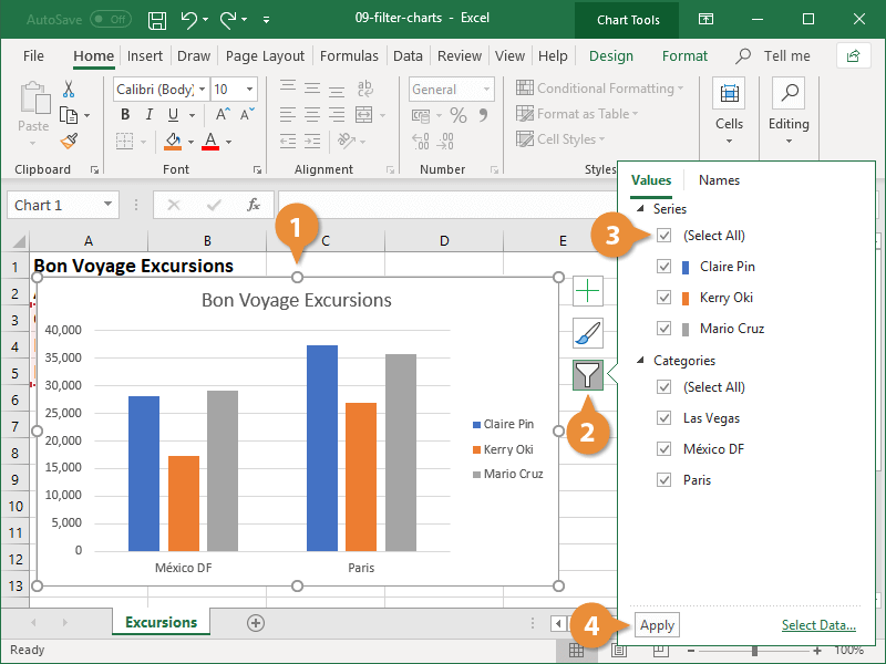
You may occasionally want to turn off certain parts of your chart, to focus in on specific data. This can be accomplished with filtering.

Filter a Chart

1. Select the chart you want to filter.
2. Click the Chart Filters button.
3. Select the item(s) you want to display or hide.
4. Click Apply.
   

All the data remains in the worksheet, but only the selected values appear in the chart.

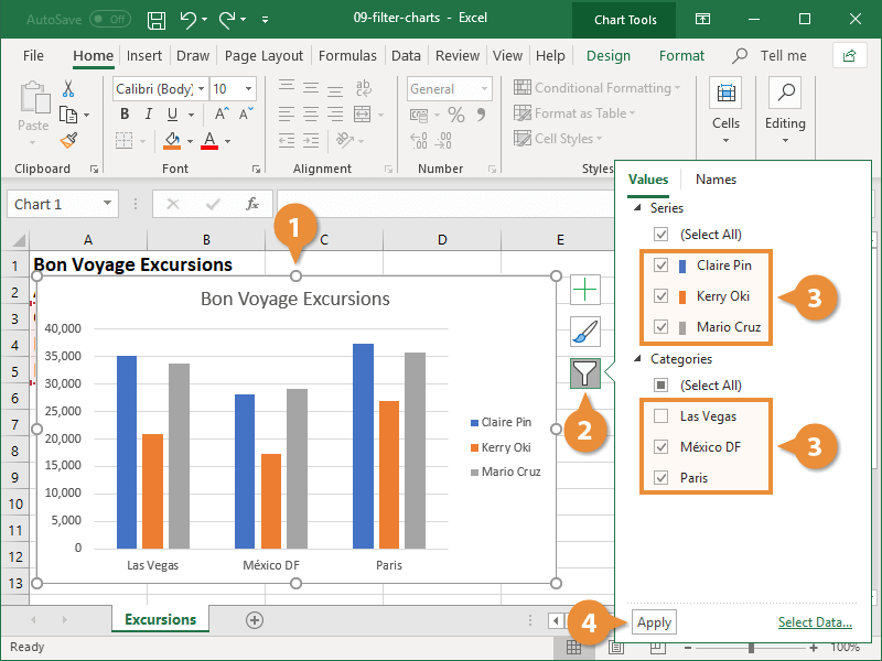
Remove a Filter

When you need to see all your data again, clear the filter.

1. Select the chart with the filter you want to remove.
2. Click the Chart Filters button.
3. For the data that’s filtered, click the Select All check box twice.

   Clicking the check box once deselects everything. Clicking it again turns everything on again.

4. Click Apply.